Model specification

Selecting a dataset

There are two ways to select the dataset for an analysis.

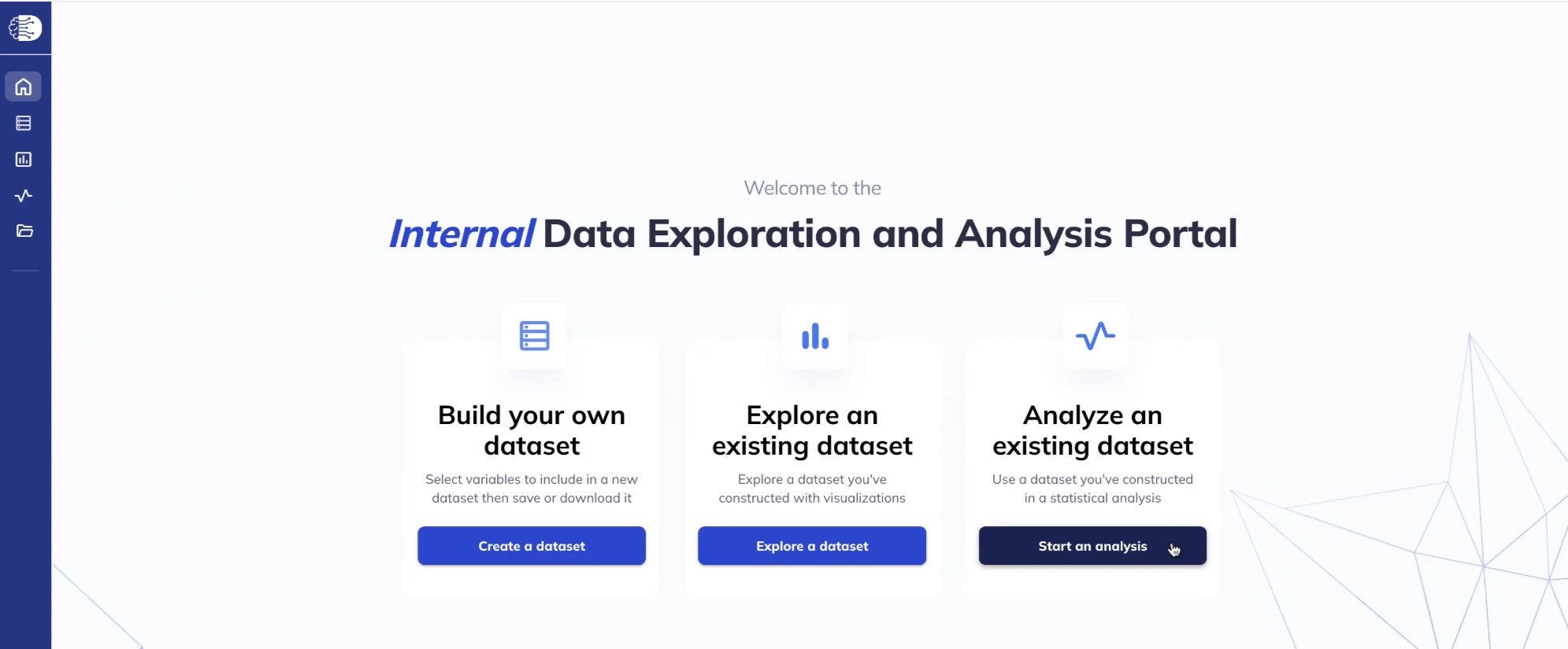
1. From the Home page

From the Home page: under the Analyze an existing dataset section, select Start an analysis.

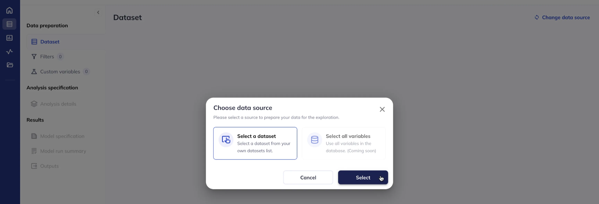
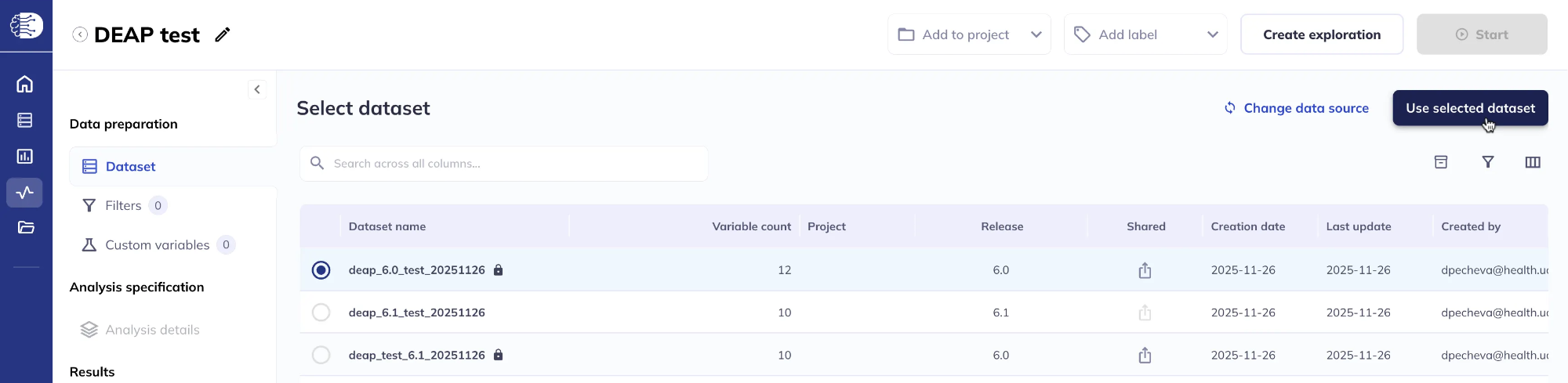
Click Use selected dataset (the Select all variables option will be available soon).

This will bring up a list of your saved datasets. Select the dataset you wish to use and click Use selected dataset.

2. From My Datasets

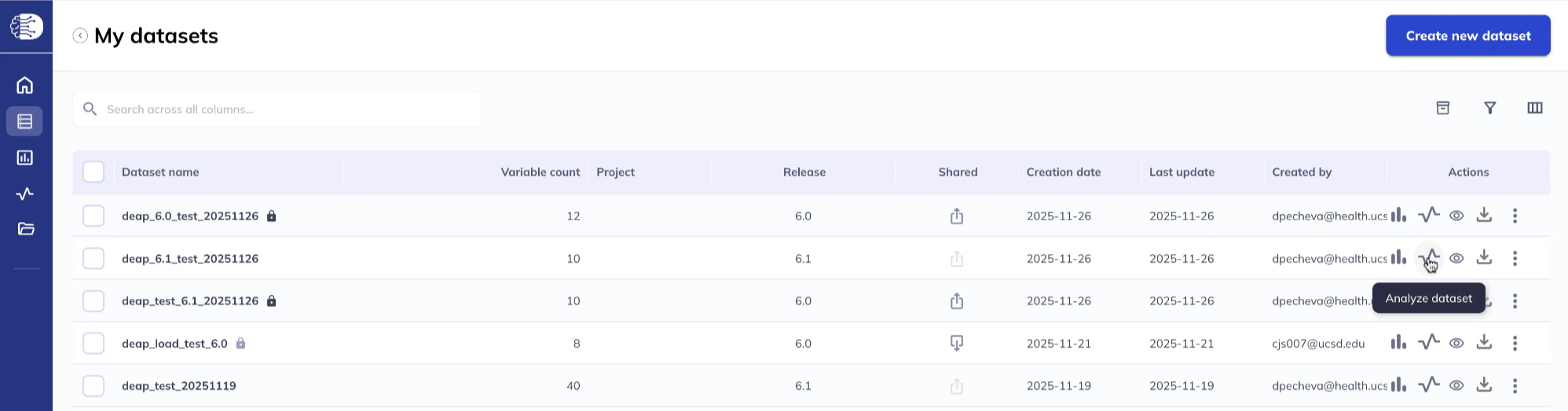
Navigate to My Datasets which will list all of your saved datasets, select one, and click the Analyze dataset icon.

Filtering the dataset

If you would like to restrict your analysis to a subset of participants/sessions, you can filter your dataset. Use a series of AND / OR statements, as well as nested groups, to limit the sample you wish to analyze. The options for filtering are the same as those available for Explorations, described in detail in the Filtering section.

Specify the model

Select model type and software

Select the Analysis details tab from the left sidebar and choose FEMA to run LME model(s).

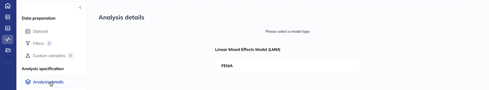
This will bring up the Analysis details page.

Specify the dependent variable(s)

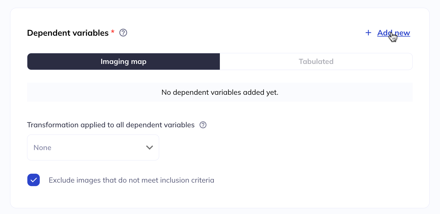
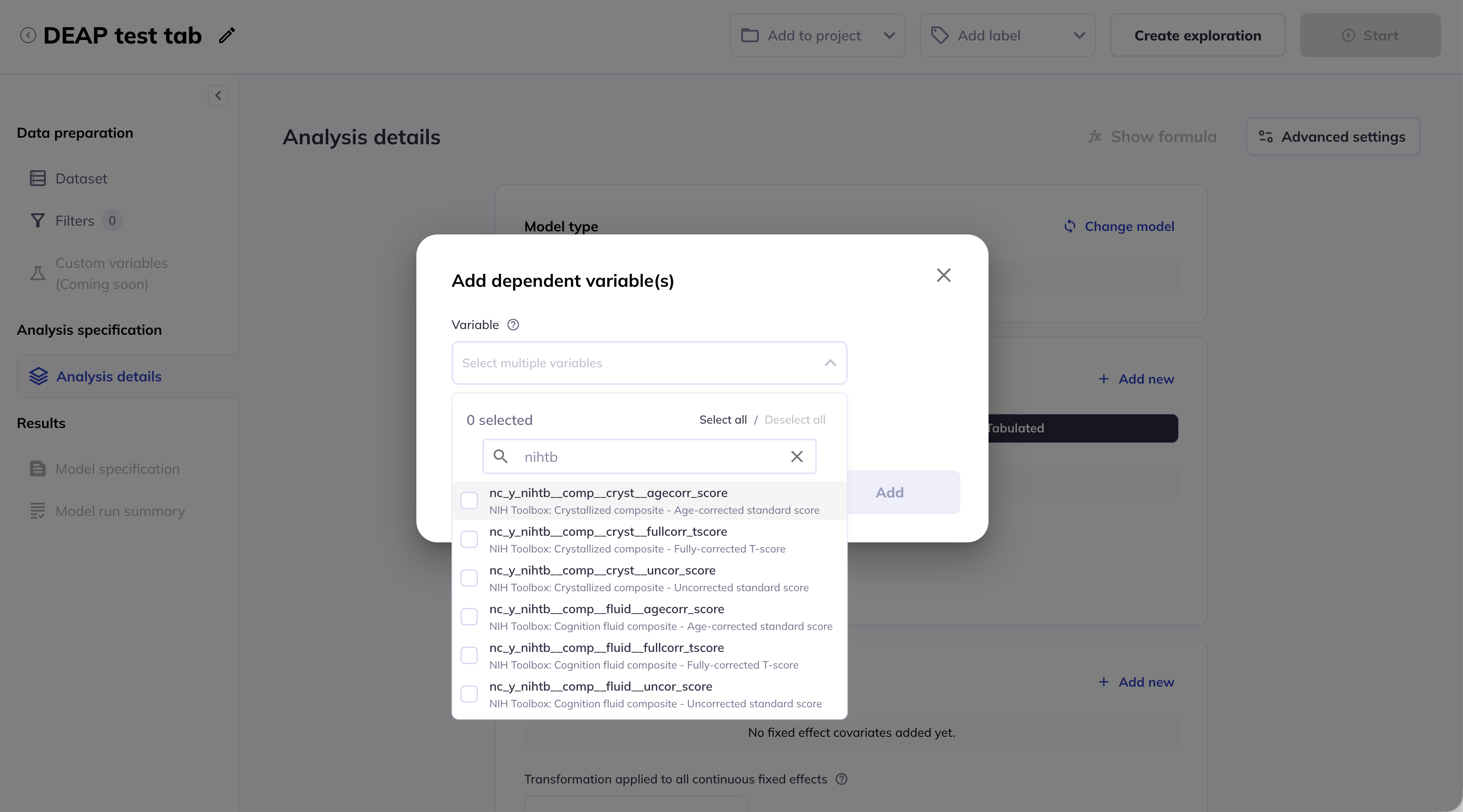
Under the Dependent variables section, click Add new to add one or more dependent variables. You can choose between Imaging map and Tabulated.

Imaging map includes whole-brain vertex-wise, voxel-wise, and ROI imaging data (connectome-wide data is coming soon). For more details on the vertex-wise, voxel-wise and connectome-wide data see the ABCD Concatenated data section in the release notes. For information on the ROI data see the Tabulated ROI-based Analysis section in the release notes.
Tabulated includes all tabulated data that are included in official ABCD releases.

Imaging map dependent variables

Variable in the Imaging map section are grouped in a nested order as follows:

modality (for example structural MRI, diffusion MRI),
measure (for example cortical thickness, fractional anisotropy),
data type (voxelwise, vertexwise, ROI, correlation matrix).

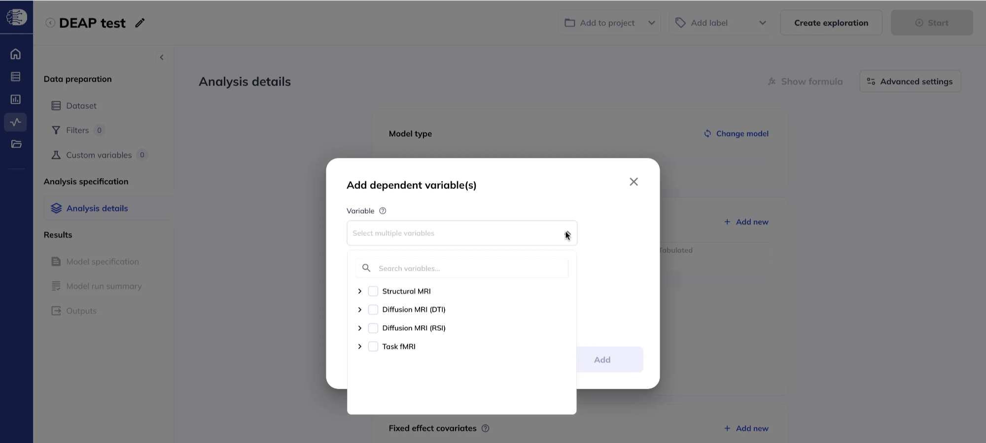
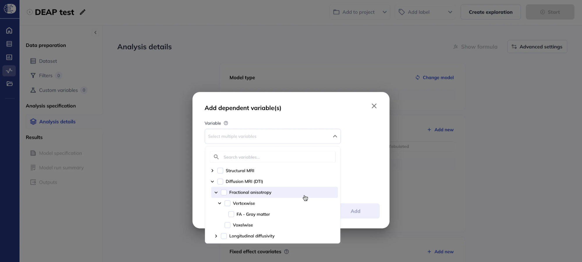
You may select one or multiple dependent variables.

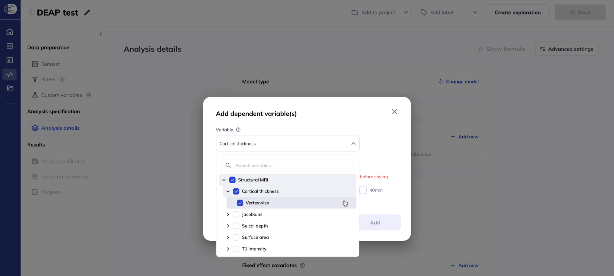
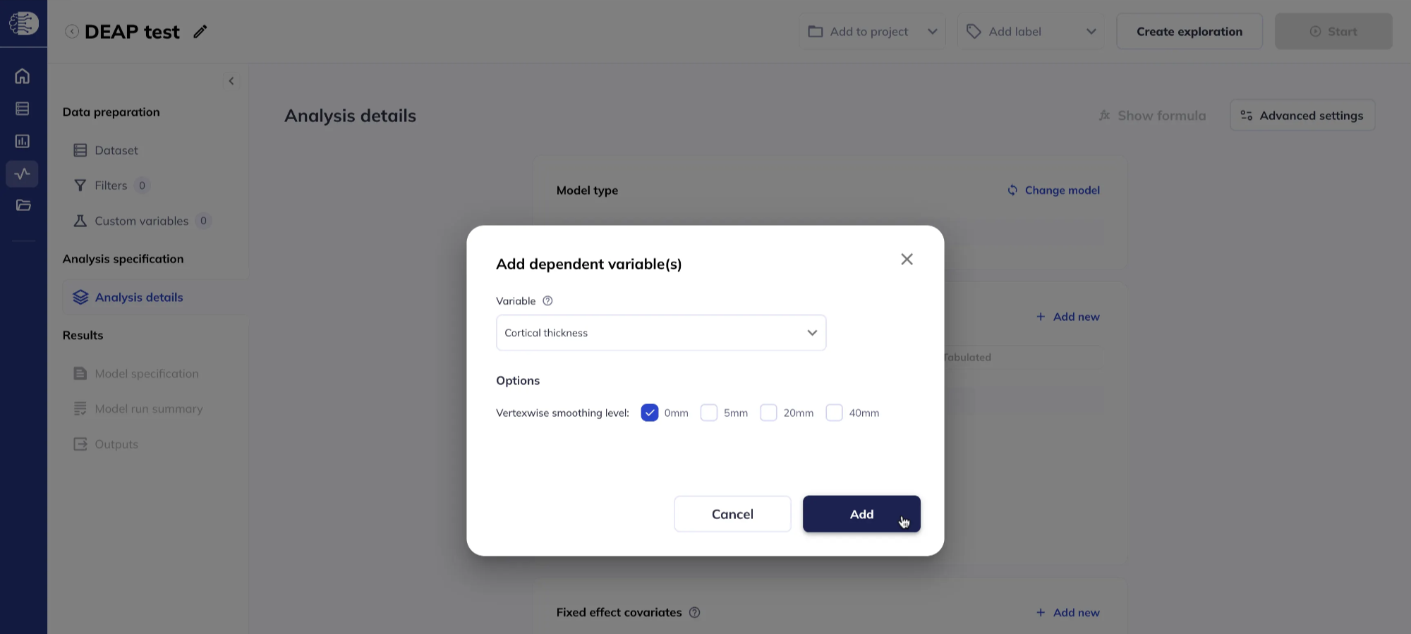
Some measures or data types have additional options which need to be specified:

For sMRI and dMRI vertexwise data, you can specify the smoothing level; choosing multiple smoothing options creates separate dependent variables for each smoothing option.
For ROI DTI data, you can choose whether to use data derived from the inner shell only or the full shell, for details see the release notes.
For fMRI data, you can choose the trimming (untrimmed, 5 minutes, 10 minutes), for details see the release notes.
For task fMRI data,
- you can choose to use either Run 1, Run 2, or All (the mean of the two runs),
- whether to use the preprocessed time series Data, task residualized time series Task-residualized, or estimated task-related time series Task-related; for details see the release notes.

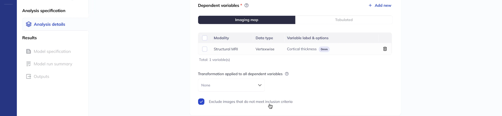
After adding variables, you can review the full list of your selections.

You can decide whether to restrict the analysis to include only scans which meet the DAIRC inclusion criteria or to include all scans.

Tabulated dependent variables

You can select one or multiple tabualted dependent variables from your datset by either scrolling through the dropdown list or using the search bar.

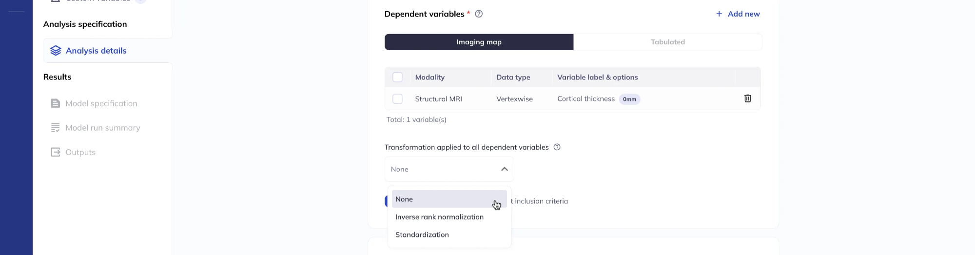
Dependent variable transformations

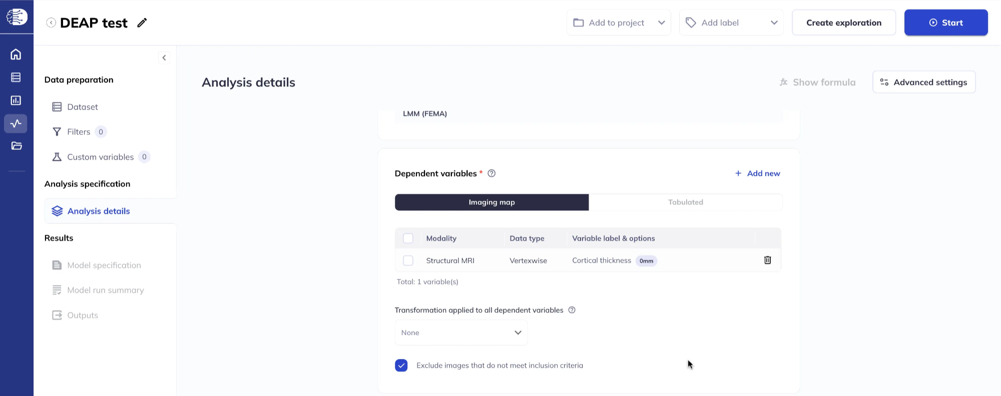
You can apply a transformation to all dependent variables according to the options presented.

Specify the fixed effect(s)

In the Fixed effects section, click Add new to add fixed effect covariates. You can select variables from your dataset.

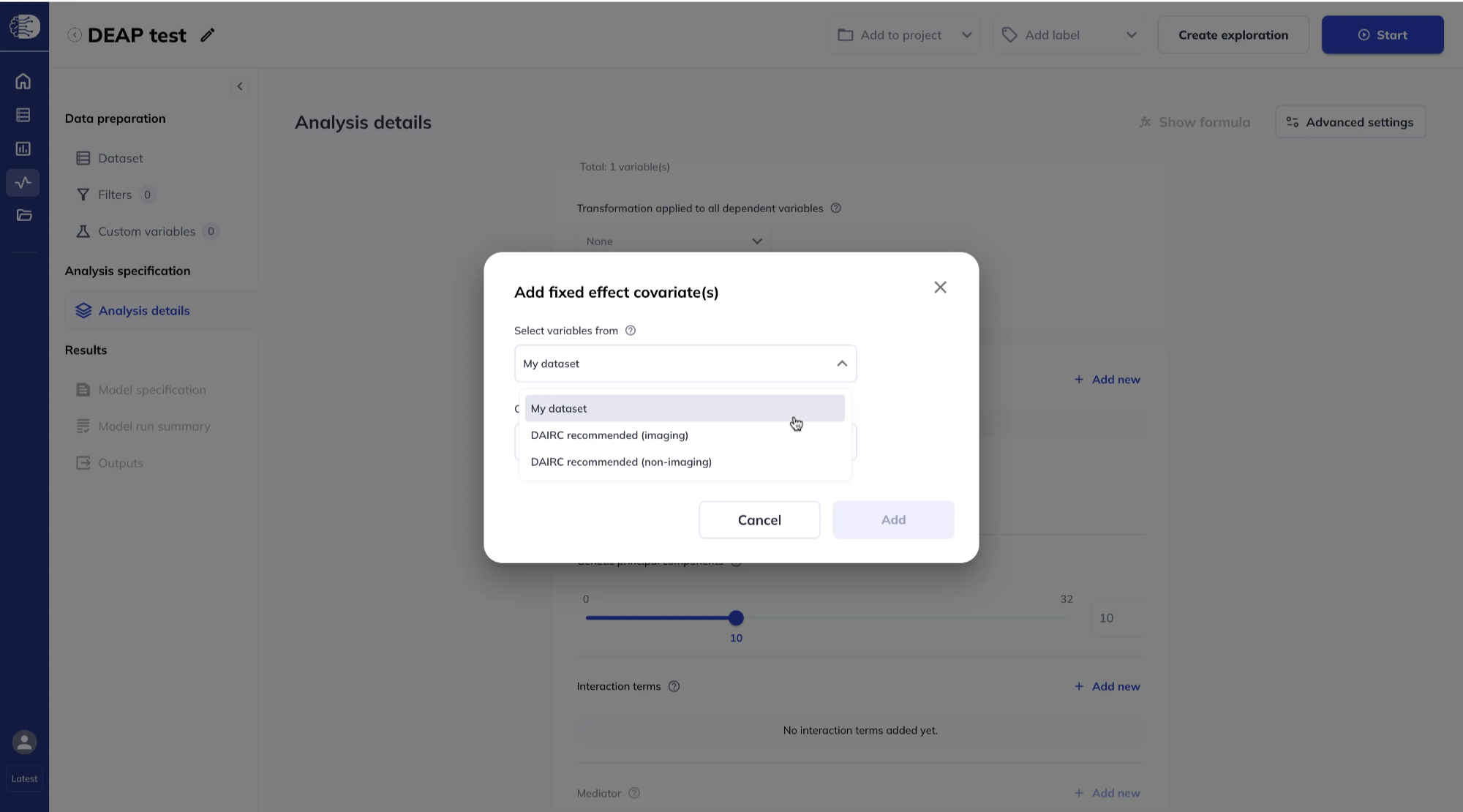
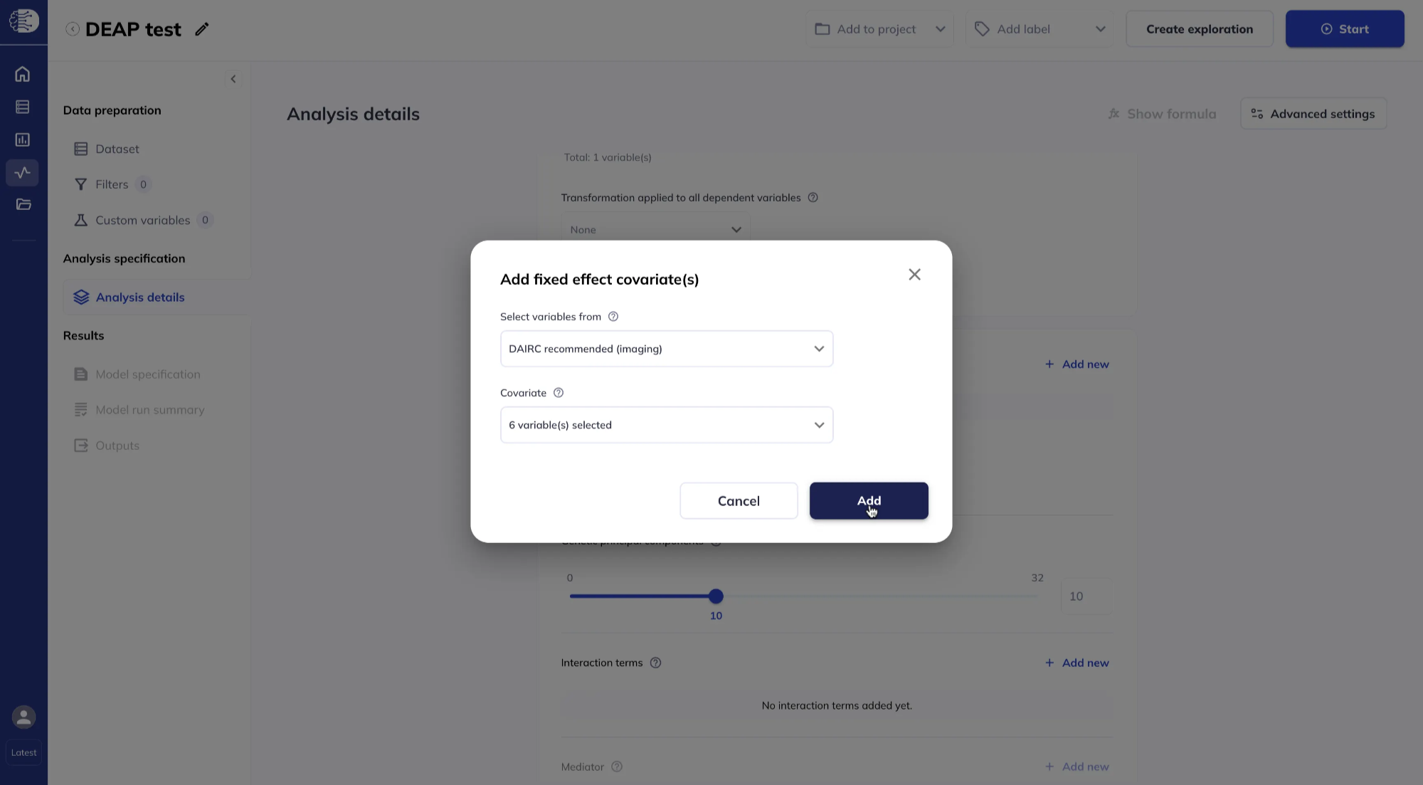
Or from DAIRC-recommended lists for imaging and non-imaging variables. If you use DAIRC-recommended variables, you do not need to have added every variable to the dataset beforehand.

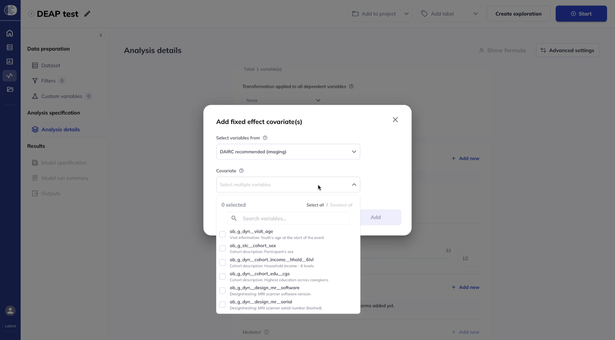
Select covariates from the dropdown list. You can add variables one at a time or click Select all, then click Add.

The interface shows a scrollable list of all the fixed effects you added.

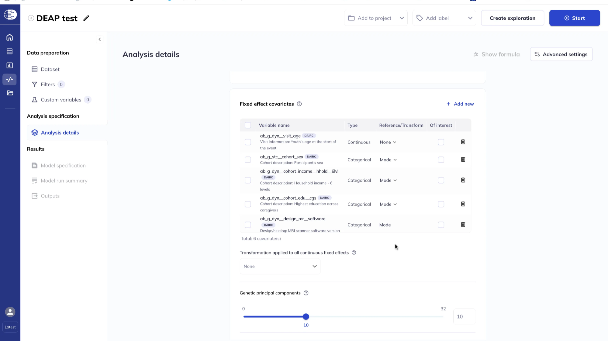
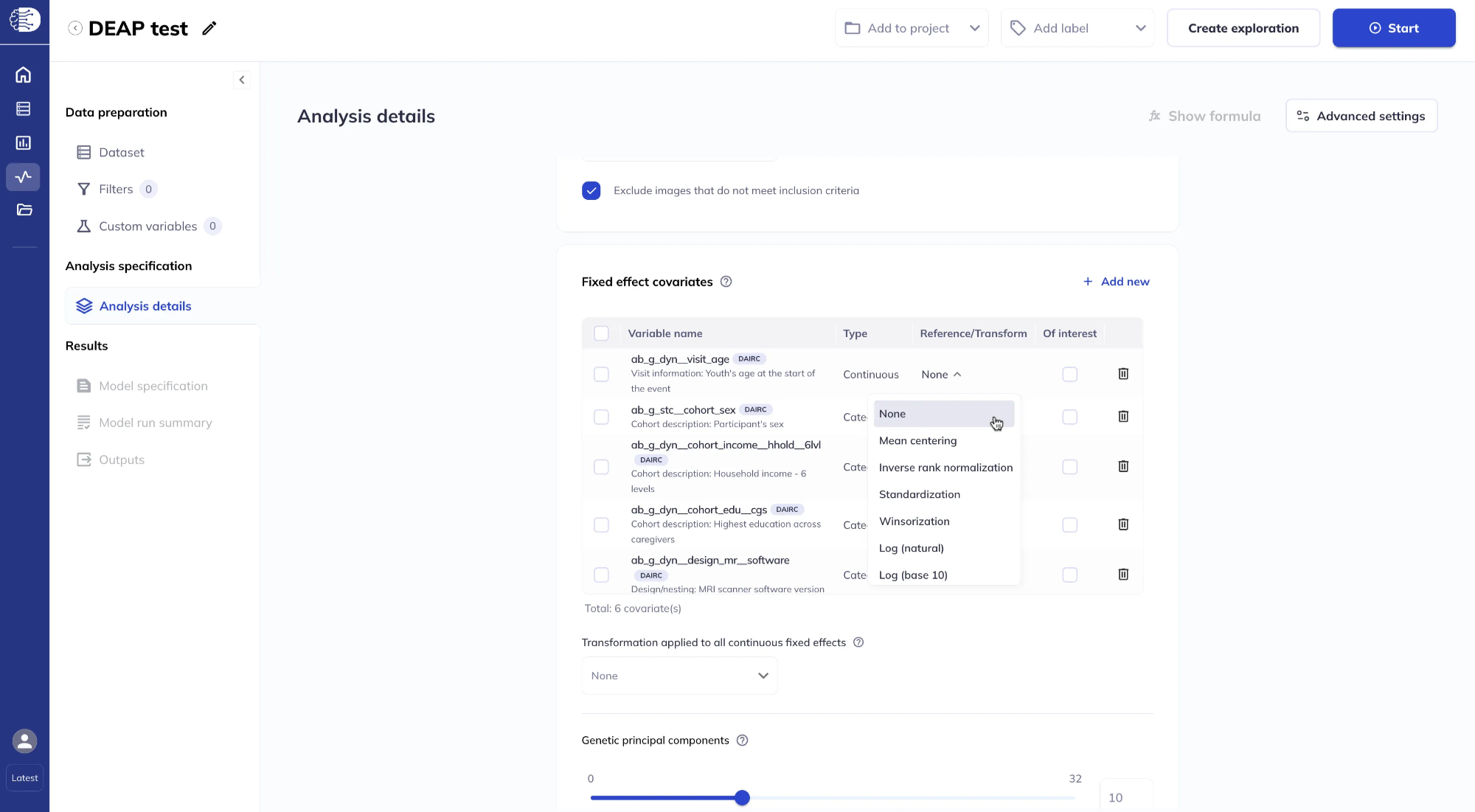
You can apply transformations to the continuous fixed effects covariates and specify the reference level for categorical variables.

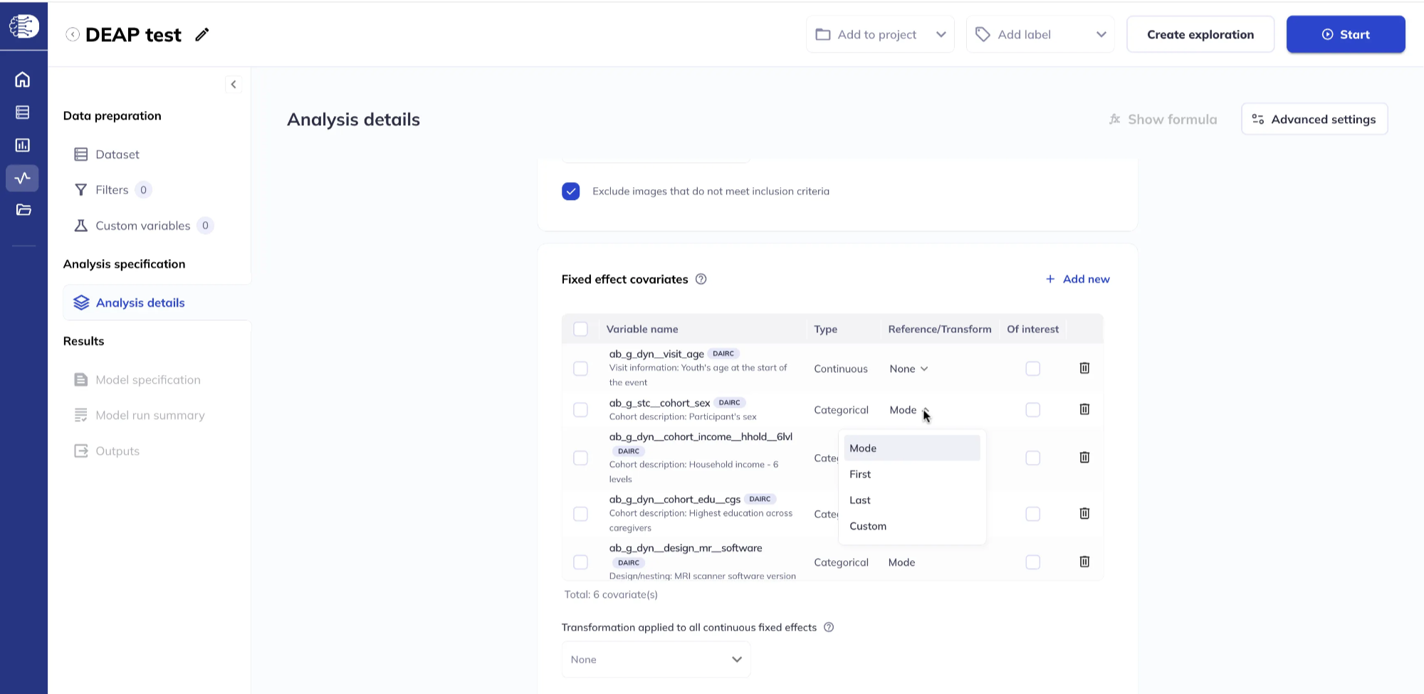
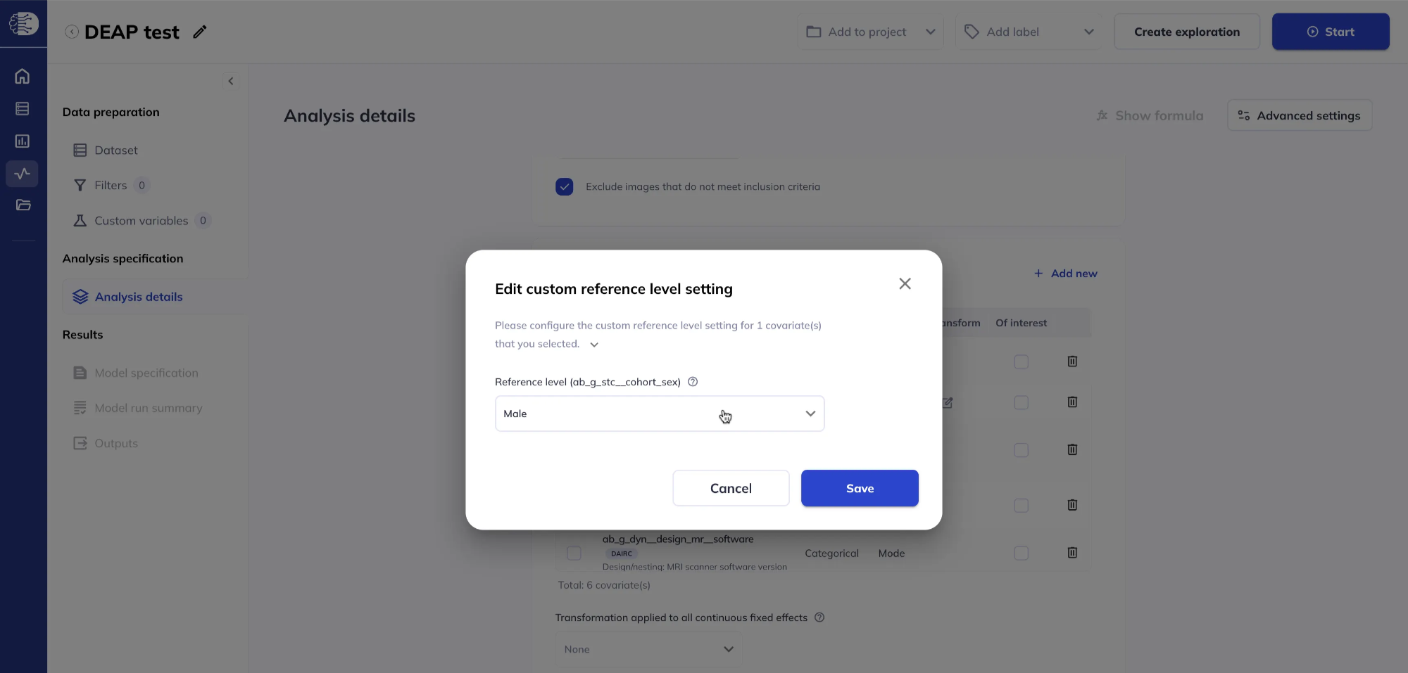
For categorical variables, set the reference level by clicking Reference/Transform. The default is Mode; other options include First, Last, or Custom. Selecting Custom opens a dialog to pick the reference category explicitly.

For continuous variables, clicking on Reference/Transform opens a dialog to choose a transformation (for example Winsorization or Splines to model the variable as a smooth function). These options may ask for extra parameters; if you leave them blank, defaults apply. For details on modelling continuous variables with splines see the Splines guide.

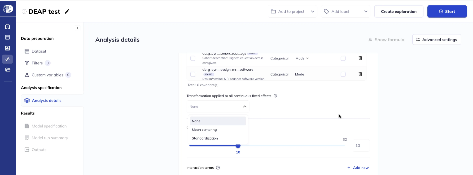
It is also possible to apply a global transformation to all continuous fixed effects. If you set both a global transform and a variable-specific transform, the variable-specific transform is applied first, then the global transform.

Transform options

For continuous variables, the following transformation options are available. The notation below assumes \(X\) is a vector indexed with \(i\), and \(X^t\) indicating the transformed variable:

Transform	Explanation
`None`	Leave the variable untransformed (default)
`Mean centering`	Subtract the mean of the variable, resulting in demeaned (zero mean) variable: \(X_i^{t} = X_i - \bar X\)
`Inverse rank normalization`	A rank-based transformation that involves computing the (tied) rank of the variable `r`, normalizing it by sample size `N+1`, and then computing the inverse of the normal cumulative distribution function of the normalized value, using zero mean and unit standard deviation: \(X_i^{t}= \Phi^{-1}\frac{r_i}{N+1}\)
`Standardization`	Subtract the mean of the variable, followed by division by the standard deviation, resulting in a variable that has zero mean and unit standard deviation \(\sigma\) (sometimes referred as normalization): \(X_i^t = \frac{X_i - \bar X}{\sigma(X)}\)
`Winsorization`	A transformation that clips the lower/upper bound of the data based on percentiles. Given a lower percentile bound \(P_{\text{lower}}\) and an upper percentile bound \(P_{\text{upper}}\), \(X<P_{\text{lower}}\) will be replaced by \(P_{\text{lower}}\) and \(X>P_{\text{upper}}\) will be replaced by \(P_{\text{upper}}\)
`Log (natural)`	Computes the natural logarithm of the variable: \(X_i^t=\ln(X)\)
`Log (base 10)`	Computes the logarithm of the variable using base 10: \(X_i^t=\log_{10}(X)\)
`Baseline-Longitudinal effect`	Transforms a vector \(X\) into a matrix with two columns: the first column is the `baseline` effect of the variable (value of \(X\) at the first event) and the second column is the `longitudinal` effect of the variable (the change in \(X\) between `baseline` and all following events)
`Quadratic`	Transforms a vector \(X\) into a matrix with two columns: the first column is the variable \(X\), and the second column is the squared value \(X^2\)
`Splines`	Compute smooth basis functions of \(X\); see the Splines guide for more details

Variables of interest

When analyzing Imaging map dependent variables, statistical maps will only be output for effects marked Of interest.

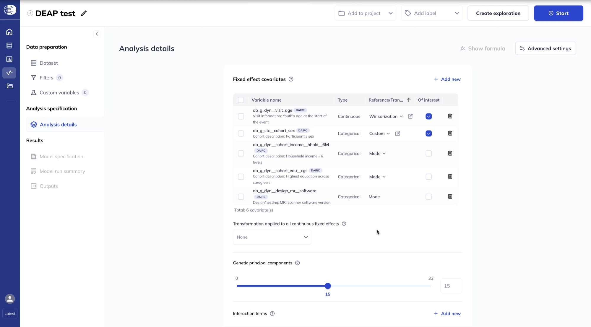
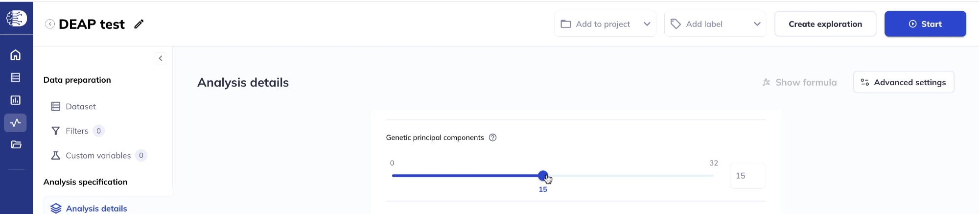
Genetic principal components

You can include up to 32 genetic principal components as fixed effect covariates using the slider or entering the number directly in the box. These PCs do not need to have been added to your dataset beforehand.

Interaction terms

Click Add new in the Interaction terms section to add interactions among fixed effects you already specified.

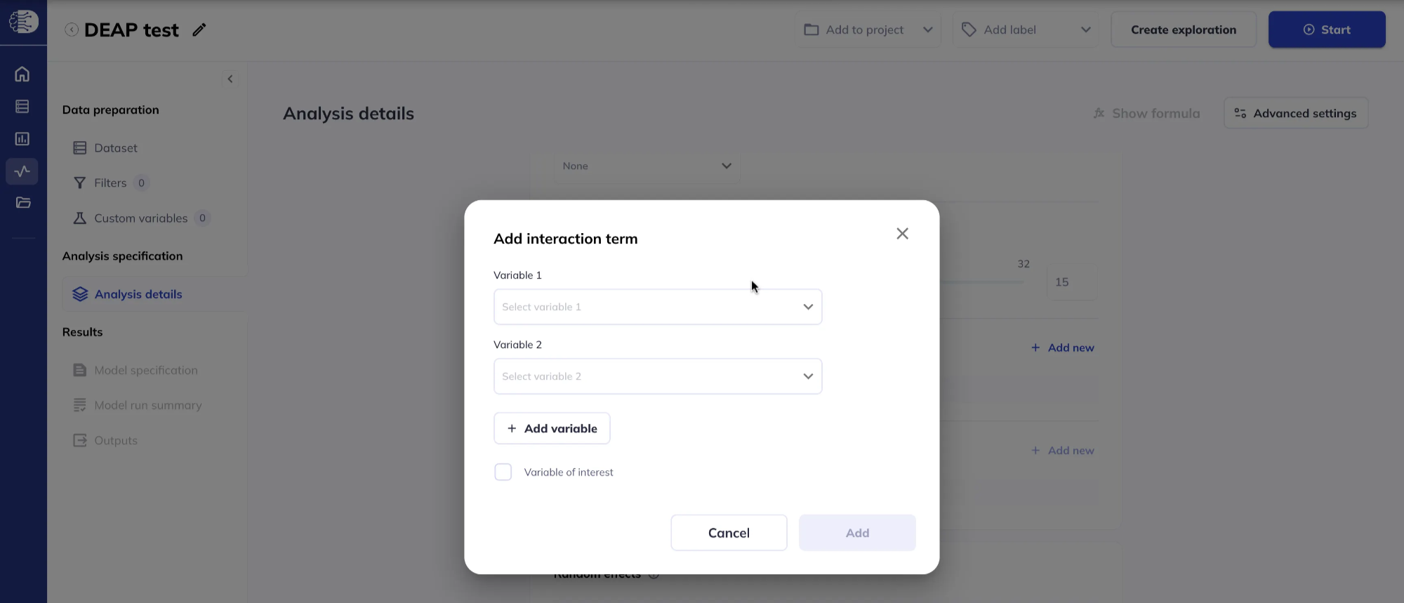
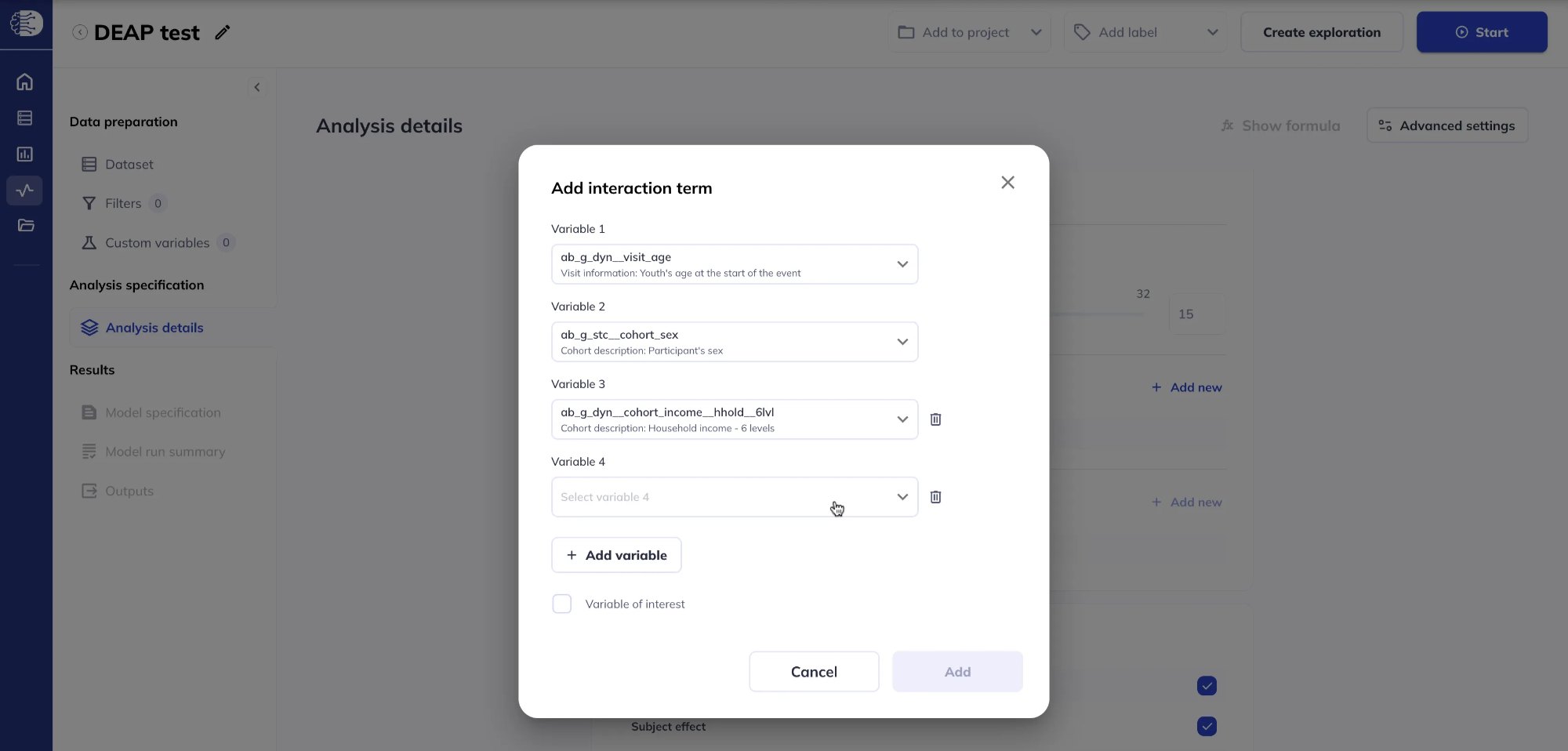
The default is a two-way interaction; click Add variable to build higher-order (n-way) interactions. Mark whether each interaction term is a variable of interest when prompted.

N.B. when creating higher-order (n-way) interactions, lower-order interactions are added automatically to the model (even though they are not visible in this interaction window). For example, if you specified an interaction between variables A, B, and C, then the final model will include the following interactions: A * B, A * C, B * C, and A * B * C. If the interaction is marked as Variable of interest, then the lower-order interactions are also marked as Variable of interest.

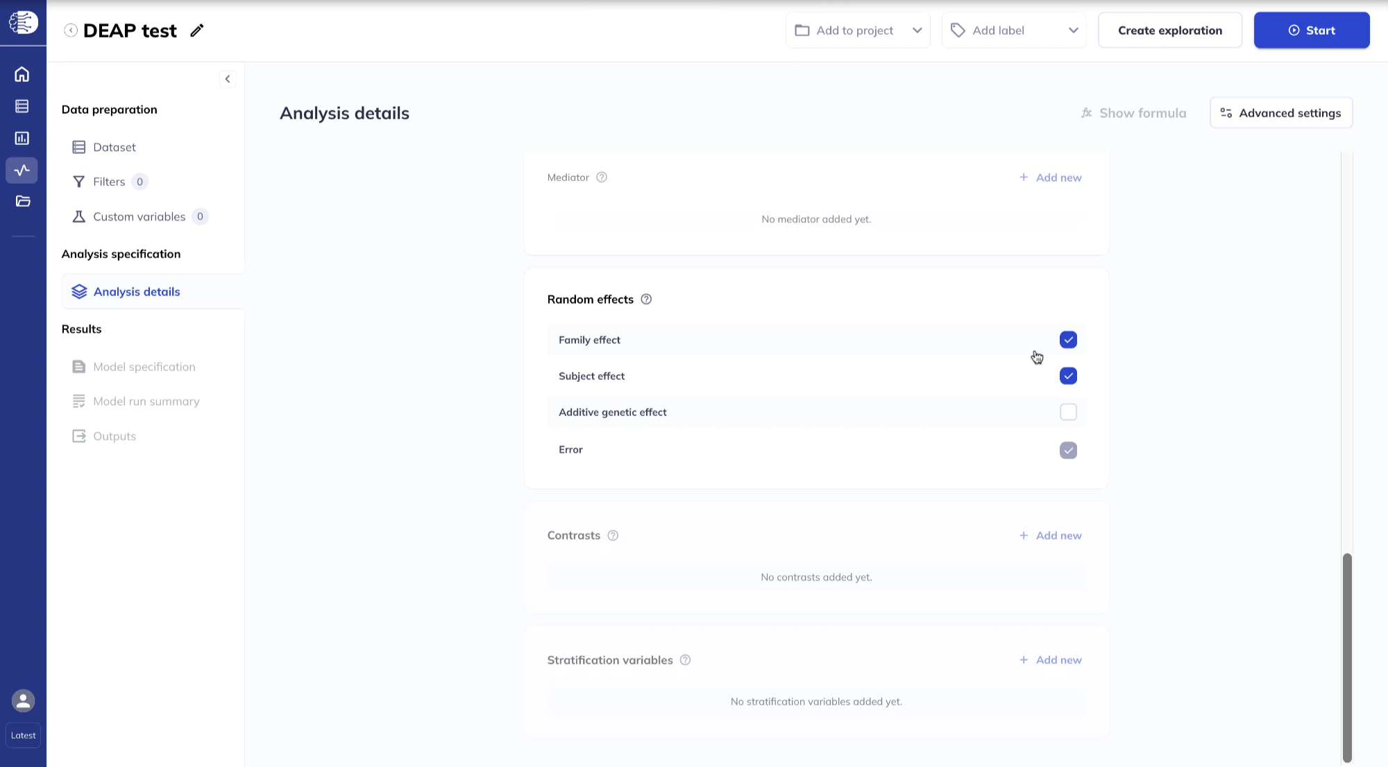
Random effect(s)

By default, FEMA specifies Family and Subject as random effects; you can include or exclude them as desired. The Additive genetic effect can also be included. The Error term can never be excluded.

Advanced settings

Click Advanced settings in the top right corner for additional options for fitting the linear mixed effects model.

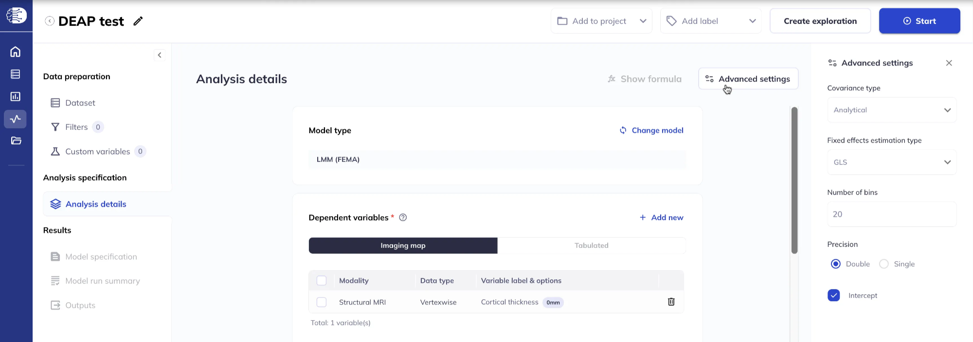
For details on the options for Covariance type, see the FEMA-long paper.

For details on the options for Fixed effects estimation type and Number of bins, see the first FEMA paper.

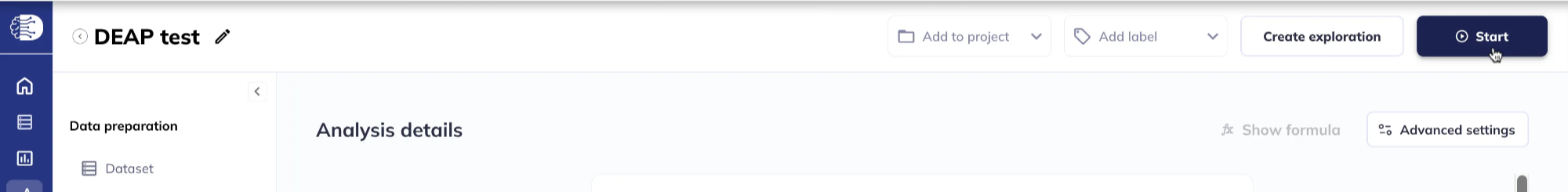
Start the analysis

Click Start to submit the analysis.

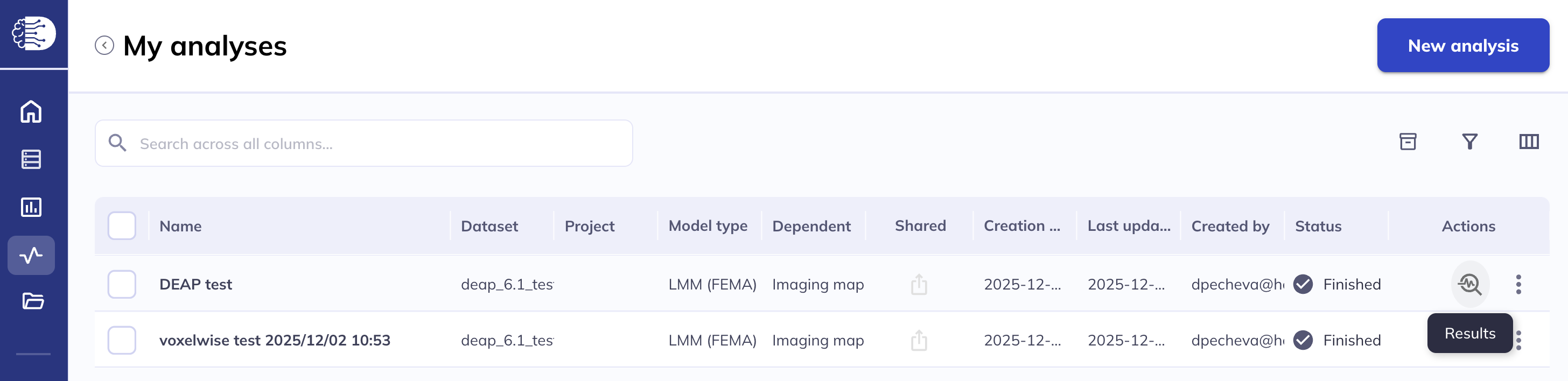
Visualizing the results

Navigate to My analyses in the left sidebar, locate your completed analysis, and click the Results icon under Actions to open the results. Depending on the data type of the dependent variables, the results will be displayed in the relevant viewer. For more details on the surface and volumetric viewers, see the Results visualization section.