Splines
Introduction
To model non-linear relationships between variables, FEMA allows any continuous variable specified as a fixed effect covariate to be modelled as a smooth function using splines.
Here we provide an overview of how spline basis functions are constructed in FEMA and the options available to the user:
- Spline type
- Method
- Powers of the variable to regress out before spline construction
- Min and max values of the variable to use
- Spline knots
If you decide to not set any of these options, FEMA will use the default settings.
Overview of spline basis function construction
When modelling a continuous variable, \(t\), with splines, FEMA represents the variable as a set of smooth basis functions. This is done by first creating \(t_{lin}\), a linearly spaced vector over the range of values in \(t\). Then smooth basis functions are created by evaluating the splines at the points in \(t_{lin}\). At this point, you have the option of regressing out powers of \(t_{lin}\). Regressing out the zeroth power of \(t_{lin}\) is equivalent to demeaning, regressing out the first power of \(t_{lin}\) is equivalent to removing the linear trend, and so on. Next, you can choose whether to perform a singular value decomposition on the basis functions to define an orthonormal basis. The orthonormal basis functions will be rescaled such that each basis function has a bounded value between [−1, 1]. Finally, whether SVD was performed or not, the basis functions are interpolated to get the corresponding basis function values for \(t\). These modified basis functions are added as columns of the design matrix. Results associated with the individual basis functions are output as <covariate>_bf1, <covariate>_bf2 etc. An omnibus Wald test is performed to test the null hypothesis that the linear combination of the estimated \(\beta\) coefficients associated with the basis functions is zero.
For a detailed description of the spline model see the Modeling spline basis functions and omnibus test section of the FEMA-long paper.
Modeling fixed effect covariates as splines
To model a fixed effect covariate as splines, under the Reference/Transform column of the Fixed effects section, select Splines.

This will open a dialog with 5 options to specify.
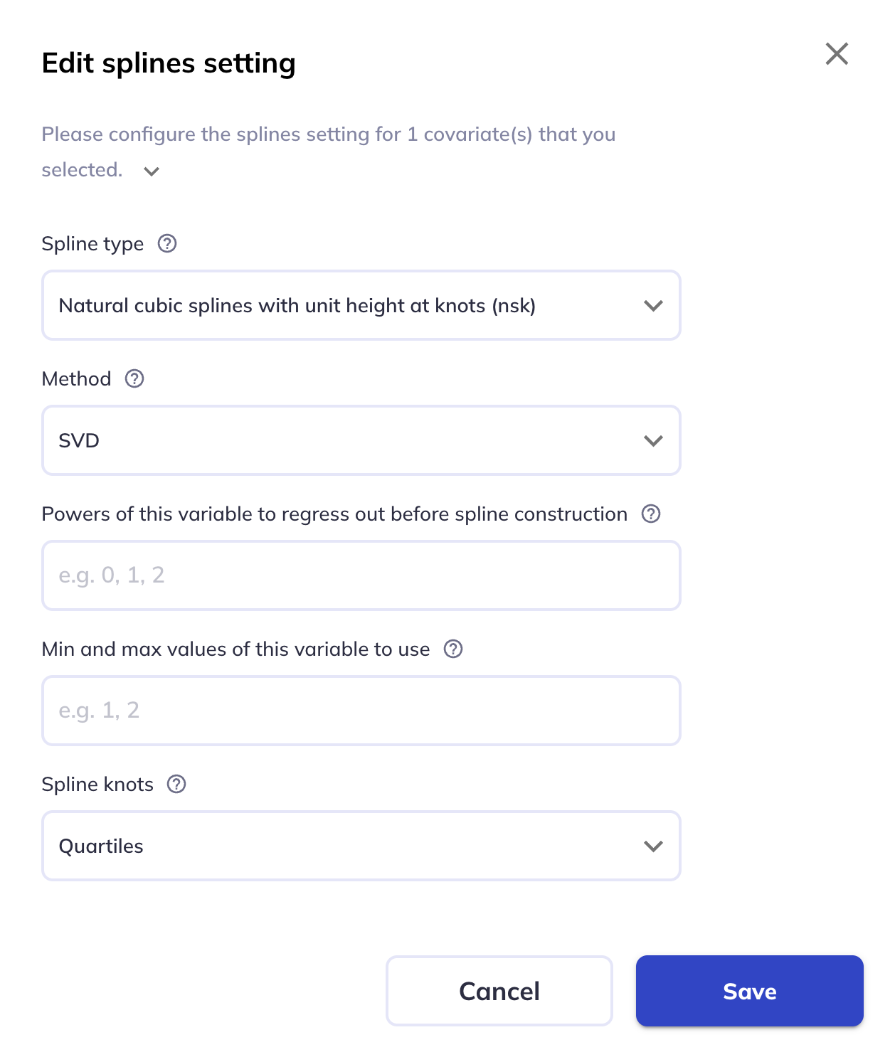
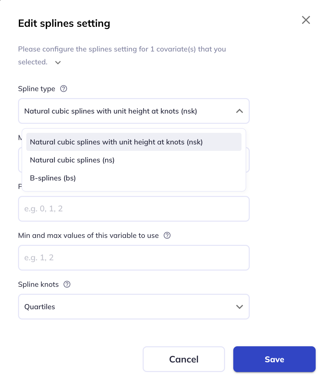
Spline type
This option specifies the type of spline to use. The options are:
Natural cubic splines with unit height at knots(default).- This is similar to the nsk option in the splines2 package in R.
Natural cubic splines.B-splines.
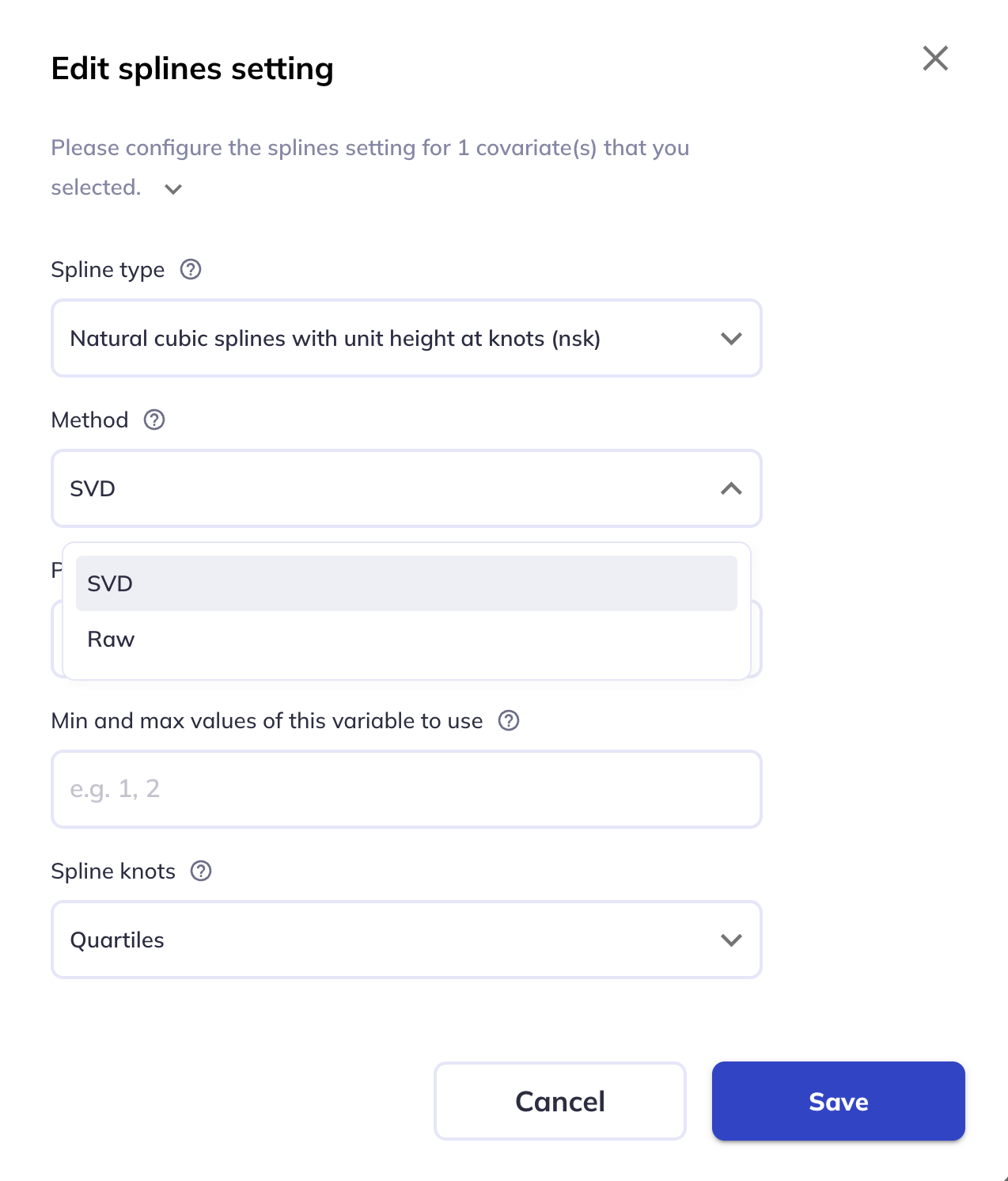
Method
This option specifies the method to use for fitting the spline. The options are:
SVD(default).- This orthogonalizes the basis functions.
Raw.- This does not orthogonalize the basis functions.
See the overview and FEMA-long paper for more details.
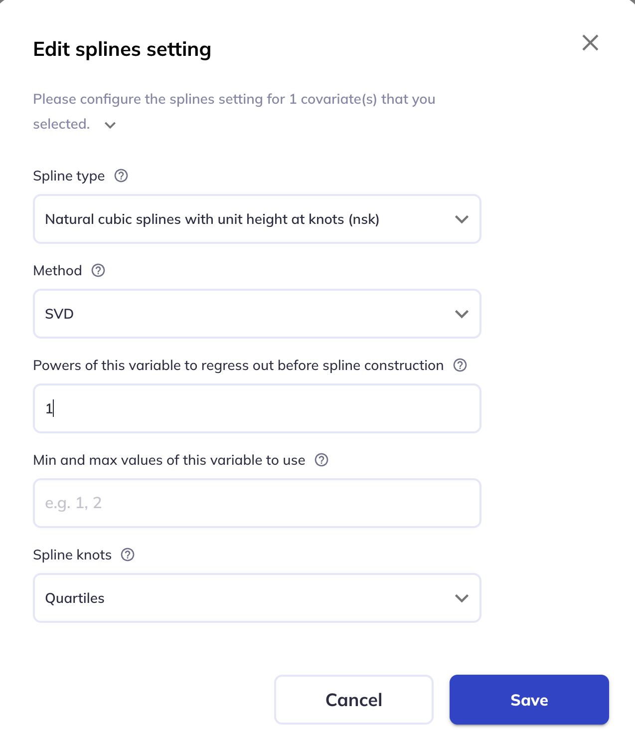
Powers of the variable to regress out before spline construction
This option specifies the powers of the variable to regress out before spline construction. You can enter any scalar value or comma-separated list of values, eg, 0,1,2 to regress out the zeroth, first, and second powers of the variable. If left blank, no powers are regressed out.
See the overview and FEMA-long paper for more details.
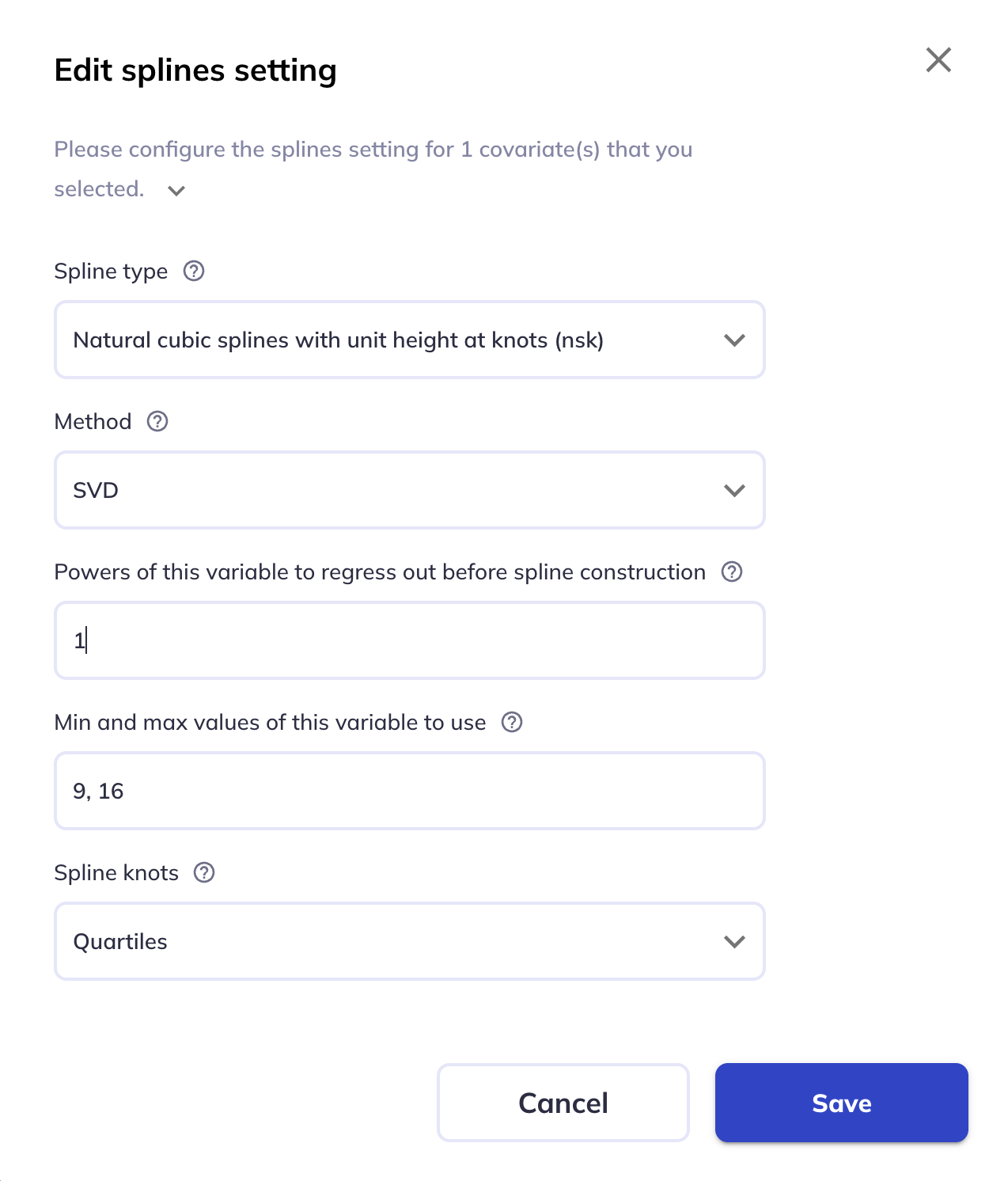
Min and max values of the variable to use
This sets the minimum and maximum values of the variable to use for spline construction. If left blank, the minimum and maximum values of the variable will be used.
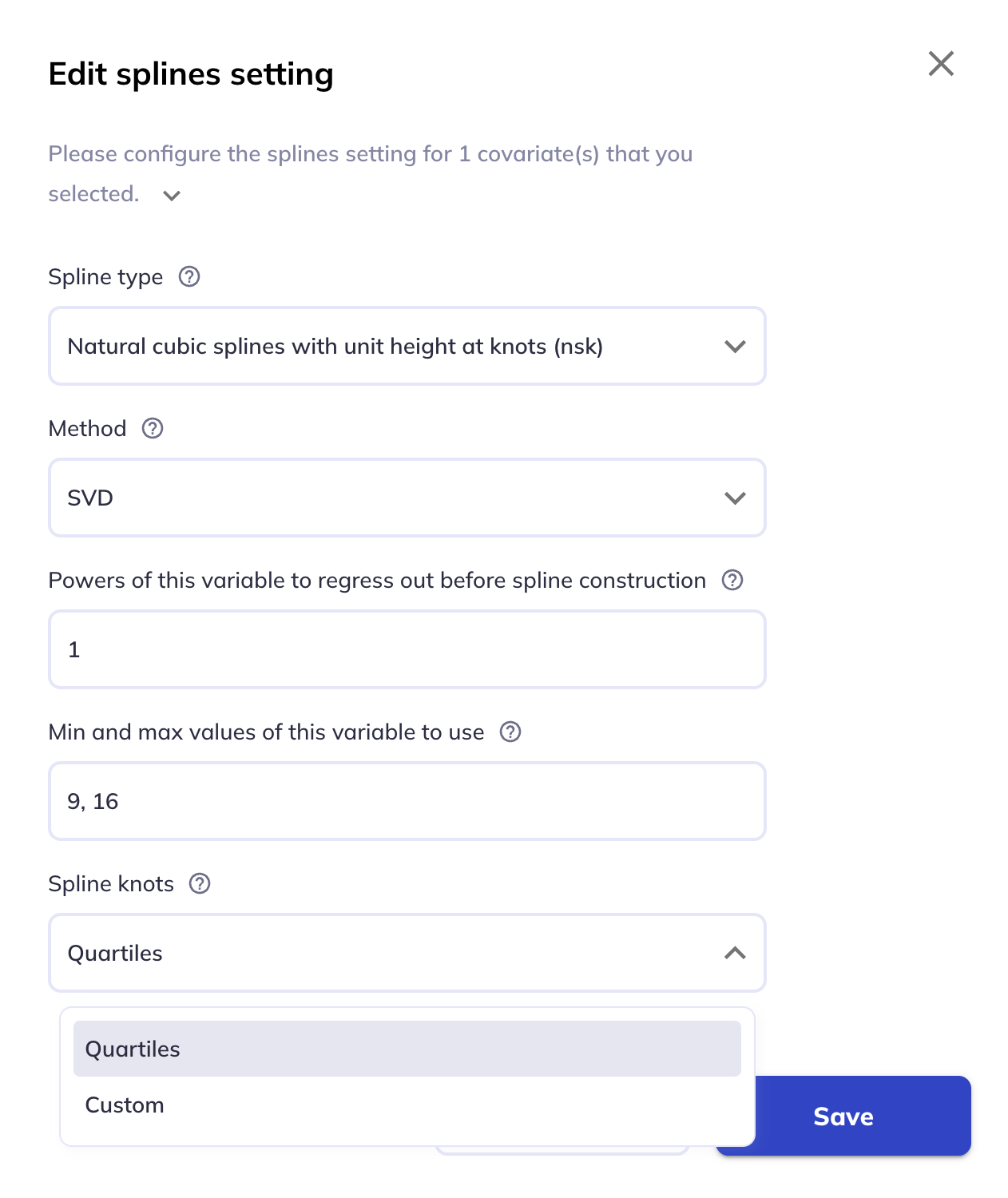
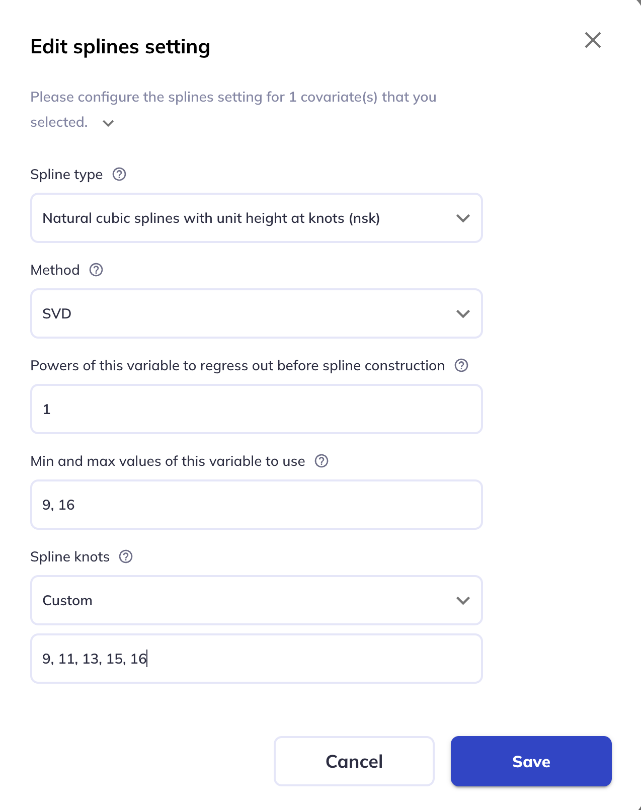
Spline knots
This sets the number of knots to use for spline construction. The options are:
Quartiles(default).- This will place the knots at the quartiles of the variable.
Custom.- This allows you to enter the knots as a comma-separated list of values.