My datasets (access & use)

To access your saved dataset, click the My Datasets () tab on the left hand sidebar. Learn more about how to manage your datasets (including, how to edit, share, organize, or download them) in the Manage tab.

Data and meta-data will change across release versions. Always confirm what release your dateset is using by checking the ‘Release’ column in My datasets.

My datasets

The My Datasets tab in DEAP serves as your central hub for managing and accessing your datasets. In this tab you get a summary view with key details about the datasets that exist on your DEAP profile. Within My Datasets you are able to organize your datasets, share datasets with others, download your datasets, and further explore your data.

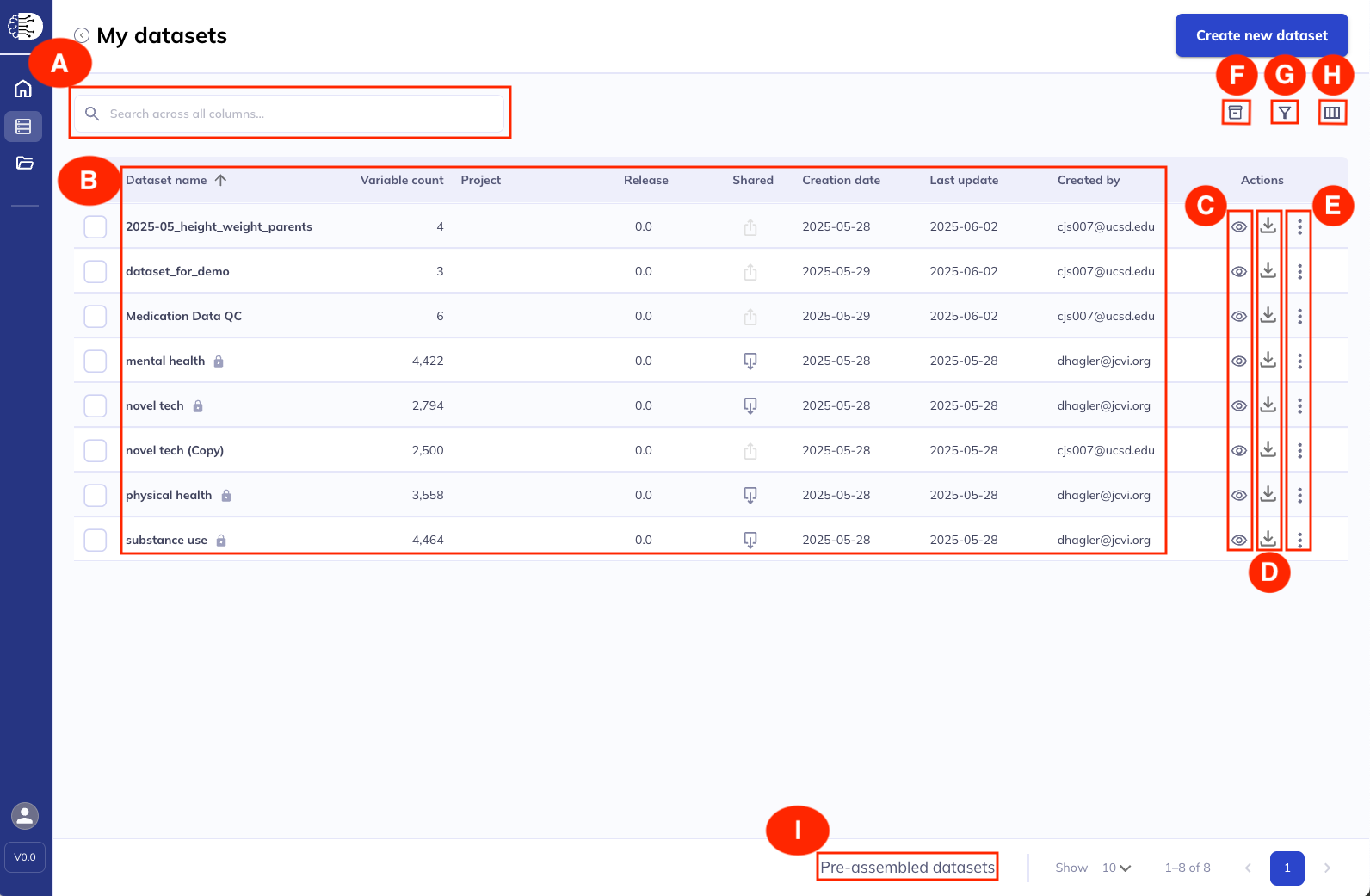
A. Search: Explore your datasets by any column displayed in the table.

B. Datasets details:

Dataset name is the name provided by the original creator of the dataset. If you are the dataset author the dataset name can be edited through the same dialog that you would edit the dataset contents. Dataset names cannot be duplicated. It is advisable that users, particularly those who use ABCD data often, name their datasets in a programmatic way, the same way you would keep files in a project on your computer organized.
Variable count displays the total current count of variables in a dataset including those added via the additional variables dialog.
Project is a user applied file organization system for datasets. Learn more about My projects here.
Release indicates the release the data originated from (e.g. 6.0 data release).
Shared uses the icon to indicate if a variable was shared with your as well as if you have ever shared the dataset.
Creation date is the date the dataset was originally set up, regardless of how many changes have been made to the dataset.
Last update displays the last time anything was done to the dataset. This includes changes to the variables set (adding, deleting variables) and organizational changes (renaming, adding to a project, editing labels, etc).
Created by helps you identify datasets you created and who shared datasets with you.

C. View datasets: Explore your dataset by clicking the icon. This view allows you to see all existing variables, edit dataset names, labels, and projects. You can also search your dataset & see the variable details. Learn more here.

D. Download dataset: To download your dataset click . This will launch a dialog box where you can modify download settings, prepare datasets for download, download the data, and access meta-data files. Learn more in the download section below.

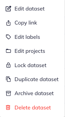
E. Additional actions: The additional actions icon () offers further actions including editing a dataset, sharing the link to a dataset, defining labels & projects, duplicating datasets, and archiving/locking/deleting datasets.

F. Archived datasets: This button () allows you to display or hide, within the main table view, datasets that you have archived. To learn more about how and why to archive datasets please review the my objects tab.

G. Filter dataset view: Similar to how you can with variables in a dataset you can also filter your displayed datasets. Like with variables, the filter function only works on columns that are currently displayed in the table (see item H).

H. Edit table view: You have the flexibility to remove and add meta-data columns to your view of the My Datasets table. For example, if you aren’t interested in the creation or update dates you can remove those columns giving more space to the information you want to visually prioritize.

Further visual table edits

Like with the data dictionary table you can edit the layout of the table.

Rearrange columns by clicking and dragging the column header around. Click between columns and drag () to change the width of columns. Click () in the column header for additional options such as sorting ascending/descending, pinning a column, filtering a column, or hiding the column. You can also select (/ ) to sort alphanumerically ascending/descending.

I. Pre-assembled datasets: Because the DEAP platform limits custom datasets to 10,000 variables and since many users may have a similar set of variables they want some pre-assembled datasets are available for expedited download. Learn more about pre-assembled datasets below.

View existing datasets

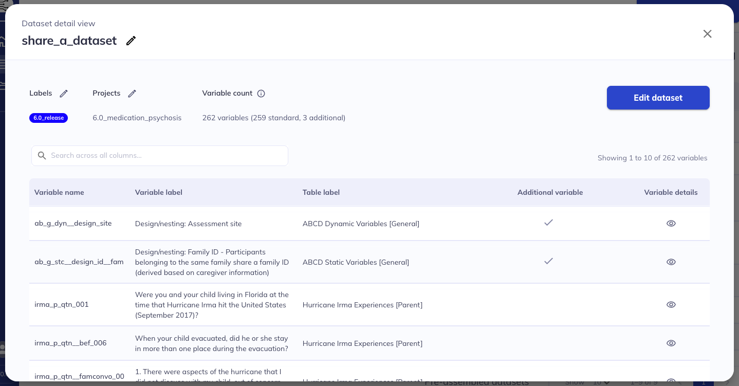
Select the icon to open your dataset details. In this pop-up you can see the number of variables in your dataset, the specific variables (variable name and label, table label, and details view), whether it was an original variable or a variable added from the additional variables dialog, and associated labels and projects. From here, you can further explore your dataset or edit it.

Edit existing datasets

From the view dataset dialog, or from the additional actions ( -> ) you can access the option to edit your existing datasets. This option will launch you back to the interface where you can create a dataset. From here you can follow the same processes as originally making a dataset for adding and removing variables.

Tip

Don’t forget to navigate to the ‘Edit and save’ tab & save your changes before exiting.

How to view and edit existing datasets

Download

DEAP allows you two pathways for accessing data: creating custom datasets tailored to specific research needs or utilizing pre-assembled datasets that contain commonly requested variable collections. For flexible use in your preferred data analysis software both download options offer up to seven file formats.

Custom datasets

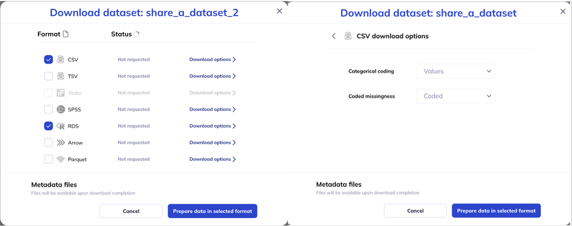
To download a dataset select in My Datasets. A dialog box will be launched where you can choose what format you would like the data to download in; to learn more about these formats visit here. Click on ‘Download Options’ to specify the coding for categories (values v. labels) and missingness (embedded codes v. NA/Null). Click ‘Prepare data in selected format’ to begin the download process.

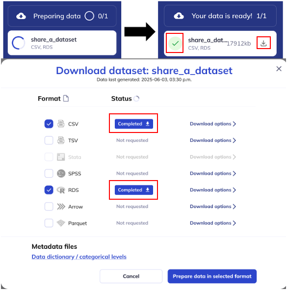
The download process will be indicated on the left hand side bar. Once the data download is complete there will be a green checkmark by your data download. You can also check on the status of the download by clicking the button again, if a download is available the status will be ‘Complete’ and a blue download button will be available. You can click either indicator to initiate the download of the data to your local folder.

The download will include 2 files, the dataset (dataset.fileformat; ex- dataset.csv) and the data dictionary (data_dictionary_levels.xlsx). The data dictionary contains all the variable meta-data for the whole ABCD study, not just the variables in your dataset. Once you have generated your dataset the metadata files will also be available in the download dialog box (pictured above).

Warning

Data and meta-data will change between release versions. Always confirm what release your dataset is composed of by reviewing the ‘Release’ column in My datasets.

Pre-assembled datasets

To accommodate users who want more than 10,000 variables, and to expedite the download of commonly requested datasets, a curated set of pre-assembled datasets has been compiled and made available on the My Datasets tab.

To access a pre-assembled dataset click the button at the bottom of the screen, select the dataset set you are interested, and the format you would like the dataset in. For pre-assembled datasets the formats and options are similar to those of custom datasets except SPSS and Stata formats are not supported. If you would like to use SPSS or Stata please use the custom dataset interface.

Available pre-assembled files:
- All variables (tables_all)
- Core (ABCD) study variables (tables_core)
- Imaging variables (tables_imaging)
- Non-imaging variables (tables_non_imaging)
- Sub-study variables (tables_substudy)
- Metadata: Data dictionary for all variables

type: Pre-assembled dataset type (all variables, imaging, etc)
file_type: Available file formats (csv, tsv, rds, parquet, arrow)
coding: output is labels or values
missing_transform: Export coded missingness as NULL/NA
size_h: human-readable size
md5: Message-digest algorithm can be used to test if the download is corrupted : Sizes are the compressed size, expect 5x+ for uncompressed files Pre-assembled data specs (6.0)

type: Pre-assembled dataset type (all variables, imaging, etc)
file_type: Available file formats (csv, tsv, rds, parquet, arrow)
coding: output is labels or values
bind_shadow: Shadow matrix included in dataset
size_h: human-readable size
md5: Message-digest algorithm can be used to test if the download is corrupted : Sizes are the compressed size, expect 5x+ for uncompressed files
Pre-assembled data specs (1.0)

Data formats & elements

Recommended format: Parquet

It is recommended that you use parquet format for tabulated data given its encoded data information (i.e. data type), compression efficiency, and faster load times.

CSV & TSV

Plain text formats (TSV/CSV) are widely compatible and easy to inspect, but less efficient for large datasets. They don’t support selective column loading or preserve metadata, such as data type specification; the metadata is instead available via the sidecar JSON files for plan text files. As a result, tools like Python or R must guess data types during import, often incorrectly. For example, categorical values like “0”/“1” for “Yes”/“No” (commonly used in NBDC datasets) may be interpreted as numeric, and columns with mostly missing values may be treated as empty if the first few rows lack data.

To avoid such issues, it’s recommended to manually define column types using the accompanying data dictionaries included in the sidecar JSON metadata files during the import. The NBDCtools R package offers a helper function, read_dsv_formatted(), to automate this process.

Stata & SPSS

Due to character limits Stata files use the column name name_stata instead of the standard variable. Stata (and SPSS) is also not available for use in the pre-assembled datasets due to their restrictions on final size; utilize custom datasets instead.

Due to character limits Stata & SPSS files use the column name name_short instead of the standard variable. Stata & SPSS are also not available for use in the pre-assembled datasets due to their restrictions on final size; utilize custom datasets instead.

Parquet

Parquet not BIDS compatible

Please note that Parquet files are not officially supported by the BIDS specification. For NBDC datasets, we decided to add Parquet as an alternative file format to the BIDS standard TSV/sidecar json pairs to allow users to take advantage of the features of this modern and efficient open source format that is commonly used in the data science community.

Apache Parquet is a modern, compressed, columnar format optimized for large-scale data. In contrast to TSV files, Parquet supports selective column loading and smaller file sizes. This improves loading speed and memory usage and enhances performance for analytical workflows.

Crucially, parquet can store metadata (including column types, variable/value labels, and categorical coding) directly in the file (as opposed to a sidecar json), enabling accurate import without manual setup. See details for how Parquet export is handled in Lasso and DEAP.

polars module:

import polars as pl
parquet_df = pl.read_parquet(
  "path/to/file.parquet"
)

pandas module:

import pandas as pd
parquet_df = pd.read_parquet(
  "path/to/file.parquet"
)

arrow package:

library(arrow)
parquet_df <- read_parquet(
  "path/to/file.parquet"
)

Shadow Matrices

Shadow matrices are currently only available for the HBCD dataset. For ABCD when downloading you can select how you would like missigness handled, coded or NULL.

Each TSV and Parquet data file in the BIDS /rawdata/phenotype/ directory has a corresponding shadow matrix file in the same format (TSV or Parquet). These shadow matrix files mirror the structure and column names of the original data files.

In the data files, missing values are represented as blank cells. Shadow matrices provide essential context by indicating the reason a value is missing (e.g., Don’t know, Decline to answer, Missed visit). Each cell in a shadow matrix corresponds to the same cell in the associated data file: If a data cell contains a value, the corresponding shadow matrix cell is blank.

If a data cell is missing, the corresponding shadow matrix cell includes a code or description indicating the reason, as illustrated below by the highlighted cells in the data file (left) vs. the corresponding shadow matrix (right).

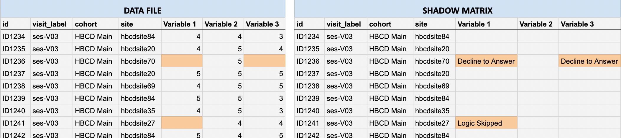
In HBCD, some participant responses like Don’t know or Decline to answer (which are typically considered non-responses) are deliberately converted to missing values in the data file, with the original response converted to a missingness reason stored in the shadow matrix. This prevents analytical errors such as inadvertently treating placeholder codes (like 777 or 999, common in other datasets) as valid numeric values during analysis and ensures consistency in data types across all entries (e.g. text notes in numeric fields are avoided).

Uses for shadow matrices {#shadow_use}

While the approach of storing missingness reasons in a shadow matrix file supports cleaner analyses, there are situations where non-responses are themselves meaningful. For example, a researcher might be interested in how often participants do not understand a given question and how this relates to other variables. In such cases, users can re-integrate the non-responses from the shadow matrix back into the data.

Utilizing shadow matrices (R & Python) {#utilize_shadow}

Here we describe how researchers can use shadow matrix files in combination with the data files to, for example, explore and understand patterns of missing data or integrate missingness reasons (e.g., Decline to Answer, Logic Skipped, etc.) into your analysis.

For working in R, we recommend using the NBDCtools package - see details here. For Python, the following helper function joins the tabulated data file with its corresponding shadow matrix file so data columns are combined with columns providing the reasons for missingness in the same data frame. This function works with both TSV and CSV file formats, but can be updated for Parquet files using the loading logic shown under the section on Parquet files above.

import pandas as pd
import os

def load_data_with_shadow(data_path, shadow_path):  
    """  
    Loads a data file (CSV or TSV) and its corresponding shadow matrix  
    (CSV or TSV) and adds '_missing_reason' columns for missing values.
    """  

    # Detect delimiter from file extension and load data
    def get_delimiter(path):
        ext = os.path.splitext(path)[1].lower()
        return "\t" if ext == ".tsv" else ","

    data = pd.read_csv(data_path, delimiter=get_delimiter(data_path))  
    shadow = pd.read_csv(shadow_path, delimiter=get_delimiter(shadow_path))

    # Annotate data with non-empty missingness reason columns (excluding participant_id 
    # and session_id) in shadow matrix 
    for col in data.columns[2:]:  
        if col in shadow.columns:
            if not shadow[col].isna().all() and not (shadow[col] == '').all():
                data[f"{col}_missing_reason"] = shadow[col]

    return data

# Example usage:
df = load_data_with_shadow("data.tsv", "shadow_matrix.tsv", save=True)

# Example: View reasons for missing data for a given column/variable in the data file 
df[df["<COLUMN NAME>"].isna()][["<COLUMN NAME>_missing_reason"]]